
Greetings, and thanks for your interest in the Sleipnir library! Sleipnir is a C++ library enabling efficient analysis, integration, mining, and machine learning over genomic data. This includes a particular focus on microarrays, since they make up the bulk of available data for many organisms, but Sleipnir can also integrate a wide variety of other data types, from pairwise physical interactions to sequence similarity or shared transcription factor binding sites. All analysis is done with attention to speed and memory usage, enabling the integration of hundreds of datasets covering tens of thousands of genes. In addition to the core library, Sleipnir comes with a variety of pre-made tools, providing solutions to common data processing tasks and examples to help you use Sleipnir in your own programs. Sleipnir is free, open source, fully documented, and ready to be used by itself or as a component in your computational biology analyses.
- Download
- Citation
- Building Sleipnir
- Example Uses
- Philosophy
- Contributing to Sleipnir
- Version History
- License
Download
- You can access the Sleipnir repository at:
https://github.com/FunctionLab/sleipnir/.
Sleipnir and its associated tools are provided as source code that can be compiled under Linux (using gcc), Windows (using Visual Studio or cygwin), or MacOS (using gcc). For more information, see Building Sleipnir and Contributing to Sleipnir.
Citation
If you use Sleipnir, please cite our publication:
Curtis Huttenhower, Mark Schroeder, Maria D. Chikina, and Olga G. Troyanskaya "The Sleipnir library for computational functional genomics", Bioinformatics 2008 PMID 18499696
Building Sleipnir
We avoid distributing binaries directly due to licensing issues, and a typical build on a "normal" desktop computer should take around an hour, but if you have problems building Sleipnir or need a binary distribution for some other reason, please contact us! We're happy to help, and if you have suggestions or contributions, we'll post them here with appropriate credit.
Prerequisites
While it is possible (on Linux/Mac OS, at least) to build Sleipnir with very few additional libraries, there are a number of external packages that will add to its functionality. A few of these are used by the core Sleipnir library, the remainder by the tools included with Sleipnir. In general, these libraries should be built and installed before Sleipnir. On Linux/Mac OS, the configure tool will automatically find them in many cases, and it can be pointed at them using the --with flags if necessary. On Windows with Visual Studio, you can use the Additional Include/Library Directories properties; see below for more details. External libraries usable with Sleipnir are:
Requirements
- GNU Gengetopt is an executable program required to build all of Sleipnir's tools. This can be compiled and installed easily on Linux/Mac OS, obtained as a binary from your favorite package distribution system, or built using Visual Studio or cygwin on Windows.
- Pthreads-w32 is required for Windows only. It is an implementation of the POSIX threads library included with Linux/Mac OS, and it can be built with Visual Studio. It should be unnecessary with cygwin.
Recommendations
- log4cpp is a logging utility used by Sleipnir to display status messages. It is available as source or binary packages for Linux/Mac OS and can be built with Visual Studio for Windows. Sleipnir will run without it, but more status information will be displayed than usual (since log4cpp filters by priority).
- SMILE is a graphical models library by the Decision Systems Library at the University of Pittsburgh. Sleipnir uses it to do most of its Bayesian analysis, so no Bayes nets will be available without it! It is distributed by the DSL as binaries built for a wide variety of platforms; if you don't see yours listed, send them an email, and they can probably help.
- SVM Perf is a support vector machine library used for SVM learning and evaluation in Sleipnir. No SVMs without it! Easily built from source under just about any environment (it's plain old C). Please note that you must use this Makefile to build SVM Perf as a library (rather than an executable) on Linux/Mac OS; in Visual Studio, set the project type to "Static Library".
Suggestions
- Readline for Windows is necessary if you're building the OntoShell tool for Windows. Linux and Mac OS generally have readline built-in, and you don't need it for any part of Sleipnir other than OntoShell.
- Boost is a huge library of C++ utilities that Sleipnir uses only to parse DOT files in the BNServer tool. Frustratingly, the DOT parser in the Boost graph library is one of the only parts that needs to be compiled (Boost is mostly a template library), but that's not so hard to do. Only needed if you're running BNServer.
Linux/MacOS
General instructions are in this section. If you want to build the latest mercurial checkout on Ubuntu, Ubuntu from Mercurial (Current as of Ubuntu 12.04) provides detailed instructions.
- Obtain any Prerequisites you need/want. These can often be installed using your favorite Linux package manager. If you need to compile/install them to a nonstandard location by hand, please note the directory prefix where they are installed.
- If you're using SVM Perf, please use this Makefile to build it as a library rather than an executable.
-
Note that SVM Perf and SMILE are both nonstandard in that they expect header files and libraries to reside in the same directory (e.g.
/usr/local/smileor/usr/local/svm_perf). - Download and unpack Sleipnir. If you elected to obtain sleipnir from the Mercurial repository, you will need to run both gen_auto and gen_tools_am (a step which requires GNU autotools).
-
In the Sleipnir directory, run
./configure. If you've installed prerequisite libraries that it doesn't find automatically, provide an appropriate--withswitch for each one. For example, to build Sleipnir with SMILE and SVM Perf installed in custom directories under -c /usr/local/, type:./configure --with-smile=/usr/local/smile/ --with-svm-perf=/usr/local/svm_perf/
-
If you'd like to install Sleipnir itself to a custom location, include a
--prefix=/custom/path/flag when you runconfigrue. -
After
configure'scompleted successfully, runmakeandmake install. - Tools that use Sleipnir will be built an installed automatically if Gengetopt and any other prerequisite libraries are available.
Ubuntu from Mercurial (Current as of Ubuntu 12.04)
-
Obtain mercurial, gengetopt, boost, log4cpp, liblog4cpp5-dev, and build-essential packages. In a terminal, type:
sudo apt-get install mercurial gengetopt libboost-regex-dev libboost-graph-dev liblog4cpp5-dev build-essential libgsl0-dev -
If desired, download and install SMILE:
-
From http://genie.sis.pitt.edu/downloads.html download the appropriate package (x64 or x86) for gcc version 4 or above (currently 4.4.5). If you have registered as a SMILE user and meet the appropriate requirements, the following commands should work for _x64 (assumes you have a Downloads directory):
  cd ~/Downloads
  mkdir smile
  cd smile
  wget http://genie.sis.pitt.edu/download/smile_linux_x64_gcc_4_4_5.tar.gz
  tar -xzf smile_linux_x64_gcc_4_4_5.tar.gz
  rm smile_linux_x64_gcc_4_4_5.tar.gz
  cd ..
  sudo mv smile /usr/local/smile
-
From http://genie.sis.pitt.edu/downloads.html download the appropriate package (x64 or x86) for gcc version 4 or above (currently 4.4.5). If you have registered as a SMILE user and meet the appropriate requirements, the following commands should work for _x64 (assumes you have a Downloads directory):
-
Currently Sleipnir requires SVMperf, so you must complete the following steps:
- Visit http://www.cs.cornell.edu/People/tj/svm_light/svm_perf.html and make sure that you meet the conditions of use (currently: "The program is free for scientific use. Please contact me, if you are planning to use the software for commercial purposes. The software must not be further distributed without prior permission of the author. If you use SVMperf in your scientific work, please cite the appropriate publications (available from the SVMperf website)").
-
Assuming you meet the conditions, the following steps in a terminal will download, compile, and install SVMperf as required by Sleipnir.
      cd ~/Downloads
      mkdir svmperf
      cd svmperf
      wget http://download.joachims.org/svm_perf/current/svm_perf.tar.gz
      tar -xzf svm_perf.tar.gz
      rm svm_perf.tar.gz
      wget http://libsleipnir.bitbucket.org/SVMperf/Makefile -O Makefile
      make
      cd ..
      sudo mv svmperf /usr/local
-
Get Sleipnir (the following assumes you want sleipnir to live in ~/sleipnir, if this is not correct, adjust the paths accordingly)
cd ~ hg clone https://bitbucket.org/libsleipnir/sleipnir -
Move to the Sleipnir directory and run the autotools scripts:
  cd sleipnir
  ./gen_auto
  ./gen_tools_am
-
Configure and build Sleipnir:
  ./configure --with-smile=/usr/local --with-svm-perf=/usr/local/svmperf/
  make
-
Assuming that all completed successfully, you can now install sleipnir to /usr/local with:
sudo make install
If you want to install sleipnir to another location, adjust the ./configure step accordingly.
Windows
This section assumes that you're building Sleipnir on Windows using Visual Studio. I'm fairly certain that Sleipnir can be built using cygwin as well by approximately following the Linux/Mac OS instructions.
-
Obtain any Prerequisites you need/want. A few of these have Windows installers, but most will need to be built using Visual Studio. In general, you can do this by:
- Unpack the library being built.
- Create an empty Visual Studio C++ project. Add all of the library's .c, .cpp, and/or .h files to the project.
- Make sure the project's Configuration Type property is "Static Library" and its Runtime Library property is "Multi-threaded" (or "Multi-threaded Debug" as appropriate).
-
Some libraries have preprocessor definitions that must be set to ensure that they are built as static libraries (e.g.
PTW32_STATIC_LIB). - Build the project.
- Download and unpack Sleipnir.
-
Open up the Sleipnir solution or individual projects. By default, Sleipnir expects external libraries to be built in a directory named
extlib. If you have built them elsewhere, make sure to update the Additional Include and Library Directories properties appropriately. - Build the Sleipnir library project first.
- If you have built the gengetopt executable in a non-default location, make sure to modify the .ggo build rule's Command Line value under the Custom Build Rules menu item.
- Build any desired Sleipnir tools.
Troubleshooting
- On Linux, when in doubt, link statically (use
LDFLAGS=-staticwhen runningconfigure). On Windows or Mac OS, when in doubt, link dynamically (e.g. in Visual Studio, using the DLL runtime libraries). Mac OS is not consistently able to link statically, and the SMILE library will only link statically in release (not debug) mode on Windows. - Choosing the correct version of SMILE can be confusing; be sure you have a recent version that matches your build environment. On Windows, this will be a version of Visual Studio (6.0 through 9.0, also known as 2008) or of gcc for cygwin. On Linux/Mac OS, this will be a version of gcc, which you can obtain with the
--versionflag. - Another charming side-effect of SMILE: any tool linked against Sleipnir in Release mode in Visual Studio must be built with the preprocessor define _SECURE_SCL=0. Since SMILE is distributed in binary form compiled with that setting, it taints anything it interacts with; building without this flag and linking against Sleipnir in Release mode will result in weird memory corruption errors when dealing with STL objects.
- Don't forget to build SVM Perf as a library rather than an executable, using this Makefile on Linux/Mac OS or setting the project type to "Static Library" in Visual Studio.
- If you're building the BNServer tool, you'll need the Boost graph library - but only the graph library! To keep from building the whole giant Boost package, try building it like this (note that the
--prefixargument is optional):./bootstrap.sh --with-libraries=graph --prefix=/desired/boost/install/path/ ./b2 install
- Pay close attention to the paths given to
--withon Linux/Mac OS and stored in the Additional Include/Library Directories properties in Visual Studio. These must point to the directories where you've installed the necessary prerequisite libraries, including both library and header files. - If you're building prerequisites by hand, you may not need to install them at all; Sleipnir can often find them if you simply point an appropriate
--withargument to the prerequisite library's source directory. - Boost again: when giving the path to the Boost libraries using
--with, beware of Boost's tendency to append the compiler version to its library names under certain circumstances. If your Boost installation includes something likegcc41in the library file names, use--with-boost-graph-libto give the path to the Boost graph library file rather than its parent directory. Remember, Boost is only used for certain tools, so it won't hurt if you need to exclude it. - If the Sleipnir tools instantaneously crash with a segmentation fault, try compiling Sleipnir and its external dependencies with
CXXFLAGS=-fno-threadsafe-statics. This works around a bug in certain versions of g++ and pthreads. - If all else fails, contact us! We're happy to receive feedback about Sleipnir, good or bad, and we're more than willing to update the code or documentation based on user contributions. If you'd like to see your name in lights on this web page, feel free to send patches, questions, or suggestions, and we'll post them whenever possible.
Example Uses
Sleipnir can be used to satisfy a variety of needs in bioinformatic data processing, from simple data normalization to complex integration and machine learning. The tools provided with Sleipnir can be used by themselves, or you can integrate the Sleipnir library into your own tools.
Tools
The following tasks are examples of what can be achieved using only prebuilt tools provided with Sleipnir. No programming necessary! To see what else can be done if you're writing your own code with Sleipnir, check out the Core Library section below.
Microarray Processing
You're investigating four different knockout strains of yeast. To assay their transcriptional response to nutrient limitation, you've grown the four cultures on media containing nothing but cheetos for two days, resulting in four two-color microarray time courses. Rather than using a pooled reference, you've used the zero time point of each time course as its reference. This leaves you with four PCL datasets, each containing twelve conditions, and each using a different reference. Your microarray technique is good but not great, so there are some missing values, and the different reference channels make it difficult to compare the different datasets. What can you do?
- Let's assume you have the datasets in four PCL files named for the gene knockouts:
pza1.pcl,ber1.pcl,rmn1.pcl, andcke1.pcl. First, use KNNImputer to impute and remove missing values for each file:KNNImputer -i pza1.pcl -o pza1_imputed.pcl
- Now, you could concatenate all four PCLs into one using Combiner :
Combiner -o combined_imputed.pcl *_imputed.pcl
- You could hierarchically cluster this combined file (or the individual files) to view with Java TreeView using MCluster :
MCluster -o combined_imputed.gtr -i combined_imputed.pcl > combined_imputed.cdt
- If you were still concerned about the different references, you could cluster the microarrays in normalized correlation space instead. First, generate normalized correlations for each file individually using Distancer :
Distancer -i pza1_imputed.pcl -o pza1_imputed.dab
- Next, combine the four resulting DAB files using Combiner, this time averaging pairwise correlation scores rather than concatenating PCL files:
Combiner -t dat -o combined_imputed_normalized.dab *_imputed.dab
- Finally, cluster the expression data using these normalized scores rather than the non-normalized correlations MCluster used in the last example:
 MCluster -o combined_imputed_normalized.gtr -i combined_imputed_normalized.dab
        < combined_imputed.pcl > combined_imputed_normalized.cdt
Clustering With Aneuploidies
In your previous microarray experiment, you discover that your ber1 knockout strain developed an aneuploidy halfway through your time course. The end of the right arm of chromosome one was duplicated in the last six conditions, artificially doubling the expression level of all of its genes. How can you keep this huge upregulation from driving your clustering?
First, create a PCL file of weights for every gene in every condition. Let's assume your original ber1_imputed.pcl file looks like this:
 ORF    NAME    GWEIGHT TIME1   TIME2   ... TIME12
 EWEIGHT            1   1   ... 1
 YAL001C    TFC3    1   0.1 0.2 ... 0.12
 YAL002W    VPS8    1   -0.1    -0.2    ... -0.12
 ...
 YAR070C    YAR070C 1   1.1 1.2 ... 1.12
 YAR071W    PHO11   1   2.1 2.2 ... 2.12
 YAR073W    IMD1    1   -1.1    -1.2    ... -1.12
 YAR075W    YAR075W 1   -2.12   -2.11   ... -2.1
 ...
 YPR203W    YPR203W 1   0.12    0.11    ... 0.1
 YPR204W    YPR204W 1   -0.12   -0.11   ... -0.1
The four YAR genes listed here have been duplicated, and their expression levels are correspondingly high. Create a weights PCL file with exactly the same structure, save that the expression values are all replaced by the desired weights of each gene in each condition. A weight of 1.0 means that the gene should be counted normally, a weight of 0.5 means that it should contribute half as much weight, 2.0 twice as much, and so forth:
 ORF    NAME    GWEIGHT TIME1   TIME2   ... TIME12
 EWEIGHT            1   1   ... 1
 YAL001C    TFC3    1   1.0 1.0 ... 1.0
 YAL002W    VPS8    1   1.0 1.0 ... 1.0
 ...
 YAR070C    YAR070C 1   1.0 1.0 ... 0.5
 YAR071W    PHO11   1   1.0 1.0 ... 0.5
 YAR073W    IMD1    1   1.0 1.0 ... 0.5
 YAR075W    YAR075W 1   1.0 1.0 ... 0.5
 ...
 YPR203W    YPR203W 1   1.0 1.0 ... 1.0
 YPR204W    YPR204W 1   1.0 1.0 ... 1.0
Each of the four duplicated YAR genes should be assigned a weight of 0.5 in the conditions where it was duplicated; thus, the whole row for PHO11 should be:
YAR071W PHO11 1 1.0 1.0 1.0 1.0 1.0 1.0 0.5 0.5 0.5 0.5 0.5 0.5
Let's name this file ber1_weights.pcl. Now, run MCluster with the expression file and the weights file:
MCluster -o ber1_weighted.gtr -w ber1_weights.pcl -i ber1_imputed.pcl > ber1_weighted.cdt
The resulting cluster output will still contain the doubled expression values, so you can see what the genes' actual expression levels were, but they won't contribute abnormally much to the clustering.
Exploring Functional Catalogs
Suppose you've just downloaded the latest and greatest versions of the Gene Ontology, MIPS Funcat, and KEGG Orthology. You're still chasing down information on your four knockout yeast strains, so you also get the GO yeast annotations and Funcat yeast annotations. This should give you five files:
gene_ontology.oboandgene_association.sgdfor GO.funcat-2.0_schemeandfuncat-2.0_data_18052006(or something similar) for MIPS.kofor KEGG (the orthology file can be hard to find; it's on their FTP site).
Let's load them into OntoShell and look around:
 OntoShell -o gene_ontology.obo -g gene_assication.sgd -m funcat-2.0_scheme -a funcat-2.0_data_18052006
        -k ko -K SCE
This should produce a command line from which you can explore the three ontologies simultaneously:
/> ls
- ROOT
O KEGG  1517
O GOBP  6462
O GOMF  6310
O GOCC  6434
O MIPS  6773
O MIPSP 0
/> cat PHO11
YAR071W (PHO11)
One of three repressible acid phosphatases, a glycoprotein that is transported t
o the cell surface by the secretory pathway
KEGG: ko00361            Metabolism; Xenobiotics Biodegradation and Metab...
      ko00740            Metabolism; Metabolism of Cofactors and Vitamins...
GOBP: GO:0006796         phosphate metabolic process
GOCC: GO:0005576         extracellular region
GOMF: GO:0003993         acid phosphatase activity
MIPS: 01.04.01           phosphate utilization
      01.05.01           C-compound and carbohydrate utilization
      01.07              metabolism of vitamins, cofactors, and prostheti...
/> ls -g GOBP/GO:0007624
- GO:0007624         1     0     ultradian rhythm
P GO:0048511         0     1     rhythmic process
 YGL181W(GTS1,FHT1,LSR1)
For more information on specific OntoShell commands and capabilities, please see its documentation.
Suppose you've discovered four genes showing unusual activity during your cheeto time courses. Create a gene list text file for those four genes:
 YAR014C
 YNL161W
 YKL189W
 YOR353C
Suppose this is named cheeto_genes.txt. We can test for functional enrichment among this gene set across all three catalogs in OntoShell :
/> find -g -l cheeto_genes.txt 0.01
KEGG:
ko04150            0.00791035    1    1    12   1517 Environmental Information Processing; Signal Transduction; ...
GOBP:
GO:0000903         6.55773e-011  4    4    8    6462 cellular morphogenesis during vegetative growth
GO:0016049         4.14193e-006  4    4    103  6462 cell growth
GO:0008361         1.13194e-005  4    4    132  6462 regulation of cell size
...
GOCC:
GO:0030427         6.15338e-006  4    4    153  6434 site of polarized growth
GO:0005933         7.37199e-006  4    4    160  6434 cellular bud
GO:0043332         1.07503e-005  3    4    34   6434 mating projection tip
...
MIPS:
40.01              4.53959e-005  4    4    239  6773 cell growth / morphogenesis
40                 7.86743e-005  4    4    274  6773 CELL FATE
40.01.03           0.00519136    2    4    37   6773 directional cell growth (morphogenesis)
So it looks like eating nothing but cheetos has something to do with vegetative growth! You could run this same command directly from the command line to save the output in a file for later reference:
 OntoShell -o gene_ontology.obo -g gene_assication.sgd -m funcat-2.0_scheme -a funcat-2.0_data_18052006
        -k ko -K SCE -x 'find -g -l cheeto_genes.txt 0.01' > cheeto_genes_enriched_terms.txt
Bayesian Data Integration
You've done about as much by-hand analysis of your cheeto time courses as you can, so you're ready to throw some machine learning algorithms at them. Suppose you want to construct a predicted functional relationship network specific to your four datasets and the process of "cellular morphogenesis during vegetative growth".
- First, you need to assemble a gold standard listing all (or at least some approximation of) known functional relationships in yeast. The GRIFn functional slim lists several hundred GO terms known to be informative; that is, genes coannotated to these terms are likely to be functionally related. Let's turn this functional slim into a gold standard answer file. Using a text editor or Excel, flip the file's columns around and trim out extraneous data so that it has two tab-delimited columns, first the GO term name and then its ID, one per lime:
 translation    GO:0043037
 cytoskeleton organization and biogenesis   GO:0007010
 transcription from RNA polymerase II promoter  GO:0006366
 ...
 boron transport    GO:0046713
- Now, we'll turn these GO term IDs into gene sets by dumping the genes annotated to each term. Create a directory named
positivesand run BNFunc :BNFunc -o gene_ontology.obo -a gene_assocation.sgd -i GO_functional_slim.txt -d positives
- Using Answerer, we can turn these gene sets into a gold standard DAB file. Note that we're using genes coannotated to a GO term as positives and not coannotated to any GO term as negatives. See the Answerer page for more information on the
-lflag as well:Answerer -p positives -n positives -l 0.05 -o answers.dab
- You can automatically create and learn a Bayesian network that will integrate your four datasets in a context-specific manner. Assuming you've generated the four files
pza1_imputed.daband so forth in the example above, and let's add four quantization QUANT files for them and one for the answer file. The answer file's easy; it just contains 0s and 1s, so create a text fileanswers.quantcontaining one line:Since your four data files are all normalized similarity scores generated from microarrays, you can discretize them using evenly spaced bins around zero. Make four files0.5 1.5
pza1_imputed.quantand so forth, each containing the single tab-delimited line:-1.5 -0.5 0.5 1.5 2.5 3.5 4.5
- Once the five QUANT files are created, you can automatically learn a context-specific Bayesian network using BNCreator. Still got the
cheeto_genes.txtfile you created earlier? Assuming all of your files are together in the current directory, run:BNCreator -w answers.dab -o cheeto_network.xdsl -d . -c cheeto_genes.txt
- Congratulations! You've learned a Bayesian network by mining your four datasets, looking specifically for functional information pertaining to the genes of interest in your study. Let's turn it into a predicted functional interaction network by running BNCreator one more time:
BNCreator -i cheeto_network.xdsl -o cheeto_network.dab -d .
- The pairwise scores now stored in
cheeto_network.dabeach represent a probability of functional interaction between each gene pair. You can do all sorts of interesting analyses on this network, including visualizing portions of it using the bioPIXIE algorithm. If you want to see what the portion of the network around your original genes of interest looks like, use Dat2Graph :Dat2Graph -i cheeto_network.dab -q cheeto_genes.txt -k 5 > cheeto_genes_subnetwork.dot
- This DOT file can be converted into a picture using the Graphviz tools from AT&T. It should look something like this:
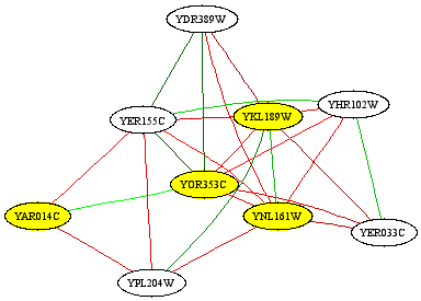
- If you want to do follow-up analysis on the predicted interaction network, you can either use the Sleipnir library to build your own tools (see the Core Library section below), or you can dump the network as text using Dat2Dab : The resulting DAT file is plain text which looks something like this:
Dat2Dab -i cheeto_network.dab -o cheeto_network.dat
 YAL001C YAL040C 0.0155878
 YAL001C YAL041W 0.242001
 YAL001C YAL056W 0.345961
 ...
- Or you might like to cluster your original microarray data using the predicted functional relationship probabilities as a similarity measure, in place of Pearson correlation or Euclidean distance. This will give you a visual representation of what transcriptional patterns look like for genes predicted to be similar based on their behaviors in your data and their relationships to your four genes of interest. If you've generated an appropriate combined PCL (see Microarray Processing ), you can run:
MCluster -o combined_imputed_fr_predictions.gtr -i cheeto_network.dab < combined_imputed.pcl > combined_imputed_fr_predictions.cdt - Or you might like to find dense subgraphs (i.e. clusters) in the predicted functional network using Cliquer : which will produce clusters and confidences resembling:
Cliquer -i cheeto_network.dab -r 3 -w 0.33 > cheeto_network_clusters.txt
 16.203  YAR071W YBR093C YHR215W YBR092C YDL106C
 14.1403 YBR066C YDR043C YHL027W YDR477W YBR112C YJL089W
 15.3548 YBR093C YML077W YML123C YHR136C
 14.1379 YIL108W YOR032C YFR028C YGL003C YGR225W
 13.2328 YMR238W YOL131W YLR295C YKL046C YDR309C YHR061C YMR055C
 ...
- Finally, you can assign predicted gene funtions by examining which genes in the network are strongly connected to known processes. Say you want to see the top 100 genes predicted to be most associated with your process of interest, the four active genes listed in
cheeto_genes.txt. Then use Hubber to run:This will result in a list of the 100 genes most confidently predicted to function with your four active genes, of the form:Hubber -i cheeto_network.dab -g 100 cheeto_genes.txt > cheeto_gene_predictions.txt
There's plenty more you can do with the Sleipnir tools to analyze interaction networks and datasets of many types - look for genetic hubs, predict associations between pathways, try out different ways of measuring protein domain similarity, or find out what biological processes are activated in your experimental conditions. To really get into the nitty gritty, keep reading to find out how you can integrate the Sleipnir library into your own computational biology tools and programs.YER033C|22.51|0 YDR389W|17.9219|0 YPL204W|16.5705|0 ...
Core Library
While the tools provided with Sleipnir satisfy a variety of common data processing needs, the library's real potential lies in its ability to be integrated into anyone's bioinformatic analyses. If you're thinking of developing your own tools using the Sleipnir library, here are some ideas.
An Important Note
Keep in mind that the best way to develop using Sleipnir is to start from one of the pre-existing tools. Copy the code and/or project file for the tool most similar to your intended goal and start modifying! This will automatically ensure that you retain the required skeleton for interacting with Sleipnir:
- Include header files for all of the classes you'll be using, and make sure you're accessing them within the Sleipnir namespace.
- Unless you're ditching gengetopts, make sure to set up your command line arguments first. An example of standard gengetopts usage is given below; if you're using something complicated like an INI file, see BNServer for an example.
- Don't forget to create a Sleipnir::CMeta::Startup before calling any other Sleipnir functions.
- Certain external libraries have their own setup/shutdown calls that need to be used separately. Older versions of SMILE use
EnableXdslFormat, for example (although it's not required any more), and on Windows, pthreads needs some setup/teardown (see below).
A skeletal main function using Sleipnir (and Windows pthreads) might resemble:
 #include "cmdline.h"
 #include "dat.h"
 #include "meta.h"
 #include "pcl.h"
 using namespace Sleipnir;

 int main( int iArgs, char** aszArgs ) {
    gengetopt_args_info sArgs;
    ... other variables here ...

    if( cmdline_parser( iArgs, aszArgs, &sArgs ) ) {
        cmdline_parser_print_help( );
        return 1; }
    CMeta::Startup( sArgs.verbosity_arg );
 #ifdef WIN32
    pthread_win32_process_attach_np( );
 #endif // WIN32

    ... do stuff here ...

 #ifdef WIN32
    pthread_win32_process_detach_np( );
 #endif // WIN32
    return 0; }
Rapid Data Mining
You've just downloaded the entire GEO database of microarrays for C. elegans. You'd like to explore these microarrays to find the gene pairs most highly correlated across the largest number of tissues.
- First, I'm afraid you'll have to do the tissue annotation youself; Sleipnir doesn't have any built-in knowledge of C. elegans anatomy! My suggestion would be to create a tab-delimited text file with one row per microarray dataset of interest and one column per condition in that dataset. In each resulting cell, use a word to summarize which tissue the condition covers (e.g. pharynx, germline, etc.)
- Let's figure out which genes are most upregulated in the intestine. Load each expression dataset into a Sleipnir::CPCL, then call Sleipnir::CPCL::Impute and Sleipnir::CPCL::Normalize. For each condition labeled as intestine in your tissue type file, remember the highest values. Then print out the appropriate Sleipnir::CPCL::GetGene names for those values. If you want, you could try using a Sleipnir::CPCLSet instead.
- Dealing with ~15,000 genes and a few hundred datasets is easy; turning those 15,000 genes into over 100 million correlations (times a few hundred datasets) is harder. At least without Sleipnir! You can convert each Sleipnir::CPCL into a symmetric matrix of pairwise correlations, a Sleipnir::CDat, using the CPCL::Distance method. Then, for each gene pair in the set of genes you've found to be upregulated in the gut, remember which ones had the highest correlation scores. You could even store that list of genes in a Sleipnir::CGenes.
- This type of analysis provides a way to rapidly uncover complex relationships in the space of gene pairs, which can be very large in higher organisms. Processing 100 million correlations over several datasets using another language or library would be slow at best; Sleipnir can find you, say, the network motif of three genes sharing the strongest average correlation in just a few minutes.
Integrative Clustering Algorithms
Want to cluster genes using more than just expression correlation? You can feed Sleipnir's built-in clustering algorithms similarity scores based on anything, or calculate your own similarity measures in real time. Here are some ideas:
- Cluster with any data you like: how about grouping genes with similar transcription factor binding site profiles? Or with high sequence similarity? Maybe shared protein domains, or all of the above?
- Add new clustering algorithms: PISA is an interesting clustering algorithm that could be extended in all sorts of ways, either by integrating different data types or by operating differently on expression data, and it would be fairly simple to implement using Sleipnir.
- Perform on the fly feature selection: add an remove microarray conditions to see which ones improve cluster cohesiveness. You could do this using an SVM or Bayes net and a functional gold standard to find out which conditions are most experimentally informative.
Continuous Bayesian Networks
Sleipnir contains rudimentary support for continuous naive Bayesian classifiers using any distribution easily fittable by maximum likelihood: normal, beta, exponential, etc. It also has limited support for using the PNL graphical models library from Intel, which supports a variety of sophisticated continuous models. Some potential avenues of interest include:
- Continuous Bayesian networks, which could be used to model arbitrarily structured continuous experimental results without the need for discretization.
- Dynamic Bayesian networks, which can be used to incorporate information about time (time courses, metabolic pathways, signaling cascades, etc.) directly into machine learning models.
- Discriminative classifiers of various sorts. These can be used (like SVMs) to potentially increase performance in a classification task without explicitly modeling the data or problem domain.
Functional Ontology Comparisons
By providing a uniform interface to a variety of functional catalogs (GO, MIPS, KEGG, SGD features, and MIPS phenotypes, to name a few), Sleipnir offers not only an opportunity for data analysis but for comparative functional annotation.
- Quickly browse uncharacterized genes in order to find promising experimental targets. Better yet, make functional predictions based on data integration and use those to direct experiments.
- Generate comparative statistics. Which genes aren't annotated in any of the common functional catalogs? Which genes are annotated in some but not others, and why? Do different functional catalogs use the same evidence for annotation? Are there pathways or processes that some catalogs describe well and others poorly?
- Perform text mining. Is there functional information in the textual descriptions of genes or functional ontology terms? What functional predictions can be made using the textual (or structural) relationships between genes and/or terms?
Philosophy
While Sleipnir includes a wide variety of data structures and analysis tools, a few formats and concepts recur frequently in its design. The most important of these is the symmetric matrix, encapsulated by the Sleipnir::CDat class. A Sleipnir::CDat represents a set of pairwise scores between genes; these can be encoded as a DAT text file of the form:
 GENE1  GENE2   VALUE1
 GENE1  GENE3   VALUE2
 GENE2  GENE3   VALUE3
 YPL149W    YBR217W 15.6
 YPL149W    YKL126W -0.62
 ...
Equivalently, a Sleipnir::CDat can be encoded as a DAB binary file, which stores identical information as a symmetric matrix (i.e. a half matrix):
| GENE1 | GENE2 | GENE3 | ... | |
|---|---|---|---|---|
| GENE1 | VALUE1 | VALUE2 | ||
| GENE2 | VALUE3 | |||
| ... |
- GENE1 through GENE3 (and the yeast ORF IDs) are unique gene identifiers. These are organism specific; you can use any identification system you like so long as it's unique per gene. We recommend ORF IDs for yeast, transcript or WormBase IDs for worm, FlyBase IDs for fly, HGNC symbols for human, and MGI IDs for mouse.
- VALUE1 through VALUE3 are any numerical scores appropriate to your data. These might be correlations in microarray data, number of shared binding partners, 1 or 0 to indicate whether two genes interact in a direct binding assay, or 1 or 0 to indicate relatedness/unrelatedness in a gold standard.
- Each gene pair should appear at most once per Sleipnir::CDat. Gene pairs need not appear, so in a genome containing genes A through C, a DAT file might contain anywhere from one to three lines for pairs A B, A C, B C, or any subset thereof.
- The gene identifiers are unordered (i.e. A B is equivalent to B A).
- Gene pairs must be distinct; that is, a gene cannot be paired with itself. This means that A A, B B, and so forth are illegal.
- Gene pairs do not have to be ordered, although they usually are in these examples for visual clarity. That is, pair GENE1 GENE2 does not have to come before GENE1 GENE3 or GENE2 GENE3, but it makes things easier to read.
Continuous values in a Sleipnir::CDat can be discretized automatically (e.g. for machine learning) using QUANT files. These are one-line tab-delimited text files indicating the bin edges for discretization. For example, suppose we have a DAT file named example.dat:
 A  B   0.2
 A  C   0.9
 B  C   0.6
We can pair it with example.quant, which will contain:
0.3 0.6 0.9
This is equivalent to the discretized scores:
 A  B   0
 A  C   2
 B  C   1
Each bin edge (except the last) represents an inclusive upper bound. That is, given a value, it falls into the first bin where it's less than or equal to the edge. In interval notation, this means the QUANT above is equivalent to (-infinity, 0.3], (0.3, 0.6], (0.6, infinity).
Generally speaking, each Sleipnir::CDat represents the result of a single experimental assay (or group of related assays, e.g. one microarray time course). A group of datasets can be manipulated in tandem using Sleipnir::IDataset, an interface made to simplify machine learning or other analysis of many datasets simultaneously. This allows you to ask questions like, "Given some gene pair A and B, how did they interact in these four assays, and what does my gold standard say about their interaction?"
For more information, see the Sleipnir::CDat and Sleipnir::IDataset documentation.
Sleipnir often uses files containing gene lists, which are simple text files with one gene ID per line:
 YPL149W
 YHR171W
 YBR217W
 ...
Other text-based files include the tab-delimited zeros or defaults file format, containing two columns, the first a node ID and the second an integer value:
 MICROARRAY 0
 TF 2
 SYNL_TRAD  1
 ...
Similarly, an ontology slim file contains one term per line with two tab-delimited columns, the first a description of some functional catalog term and the second its ID:
 autophagy  GO:0006914
 mitochondrion organization and biogenesis  GO:0007005
 translation    GO:0006412
 ...
Finally, Sleipnir also takes advantage of several predefined file formats, primarily PCLs and the associated CDT/GTR file pairing system (see Sleipnir::CPCL).
In Sleipnir's tools, standard input and standard output are used as defaults almost everywhere; a "DAT/DAB" file generally means any appropriate Sleipnir::CDat format. If standard input or output is being used, DAT formatting is generally assumed; if an explicit input or output filename is given, DAB formatting is generally assumed.
Contributing to Sleipnir
While we don't (currently) have the resources to make Sleipnir a full-blown community project, we'd love to include (with full credit, of course) any patches submitted by the community. If you're interested in developing new Sleipnir tools or library components, the following steps may be useful:
- First, let us know! We'd love to hear how people are using Sleipnir and what you plan to do with it. We're happy to answer questions and offer development tips whenever possible.
- Join the Sleipnir Google group. This is a great place to ask questions if you are having trouble with sleipnir or want to discuss its development.
- Check out our Mercurial repository at
https://bitbucket.org/libsleipnir/sleipnir/overview. Thesleipnirbranch always contains the latest development version of Sleipnir, and official versioned releases appear undertags. If you'd like to submit patches to us for inclusion in Sleipnir, please try to do so against the current development version (sleipnir). This repository ties in with our ticket system which also provides a good way to submit patches.
- Construct a patch against the Sleipnir code that includes your modifications and additions. Alternatively, if you've built an independent tool that relies on Sleipnir, we can include a link to it on the Sleipnir web site.
- And finally, let us know again! We'll do our best to include any patch or link you send us, always with full credit to the creators.
Version History
- 3.0, ***
Fix confusing documentation in Answerer - thanks to Arjun Krishnan!
Fix missingSIZE_MAXdefinition on Mac OS X - thanks to Alice Koechlin!
Fix bug in Answerer when using predefined positive pairs - thanks to Chris Park!
Add Partial Correlation Coefficient normalization to CDat and Normalizer - thanks to Arjun Krishnan!
Fix bug in weighted Pearson correlation measure - thanks to Jie Tan
- 2.1, 12-20-09
Update includes for gcc 4.3 compatibility - thanks to Casey Greene!
Addhalf2relative.rbandhalf2weights.rbscripts to MIer - thanks to Arjun Krishnan!
Fix mutual info command line option in Distancer - thanks to Arjun Krishnan!
Add MedianMultiples PCL probe resolution procedure - thanks to Matt Hibbs!
Features added to Distancer and Combiner
Added Clinician tool for testing clinical correlates with expression values
Added Filterer tool for selective data removal from DABs
Updated COALESCE algorithm to published version
Several minor bug fixes and other added features
- 2.0, 06-19-09
Added COALESCE and Synthesizer as described in Huttenhower et al. 2009.
Added SVDer - thanks to AJ Sedgewick!
Fixed Answerer usage in the documentation example - thanks to Jim Costello!
Added PCLPlotter and Matcher.
Update version dependencies for SMILE, SVM Light/Perf.
Update VS2008 build system.
Add a variety of new matrix operations and statistical functions.
Many, many bug fixes and added features!
- 1.1, 06-02-08
Added BNs2Txt and Mat2Txt tools for dumping binary Bayesian classifiers and matrices.
Improved Gene Ontology parser for compatibility with latest versions.
Added term-filtered gene counts to DChecker.
Updated BNServer for HEFalMp.
Added network analysis features to Hubber and Funcaeologist.
Add Sleipnir::Percentile and Sleipnir::Winsorize statistics functions.
Change Sleipnir::CMeta behavior to avoid the compiler optimizing out proper initialization/teardown.
Improve cmdline.[ch] file handling in Visual Studio.
Minor bug fixes.
- 1.0, 05-14-08
First publicly available version.
Added Counter tool for rapid Bayesian classifier construction/inference from raw data counts.
Separate SMILE dependent and independent Bayes net headers.
- 0.9, 04-14-08
First version made available to reviewers.
License
Sleipnir is provided under the Creative Commons Attribution 3.0 license.
You are free to share, copy, distribute, transmit, or adapt this work PROVIDED THAT you attribute the work to the authors listed above. For more information, please see the following web page: http://creativecommons.org/licenses/by/3.0/